Page 161 - Applied Statistics with R

9.2. SAMPLING DISTRIBUTION 161

y_hat = X %*% solve(t(X) %*% X) %*% t(X) %*% y
e = y - y_hat
sqrt(t(e) %*% e / (n - p))

## [,1]
## [1,] 3.431367

sqrt(sum((y - y_hat) ^ 2) / (n - p))

## [1] 3.431367

9.2 Sampling Distribution

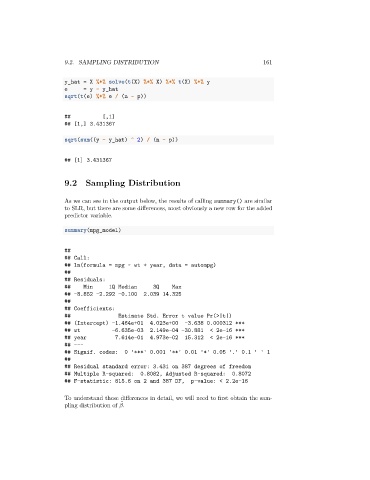
As we can see in the output below, the results of calling summary() are similar
to SLR, but there are some differences, most obviously a new row for the added
predictor variable.

summary(mpg_model)

##
## Call:
## lm(formula = mpg ~ wt + year, data = autompg)
##
## Residuals:
## Min 1Q Median 3Q Max
## -8.852 -2.292 -0.100 2.039 14.325
##
## Coefficients:
## Estimate Std. Error t value Pr(>|t|)
## (Intercept) -1.464e+01 4.023e+00 -3.638 0.000312 ***
## wt -6.635e-03 2.149e-04 -30.881 < 2e-16 ***
## year 7.614e-01 4.973e-02 15.312 < 2e-16 ***
## ---
## Signif. codes: 0 '***' 0.001 '**' 0.01 '*' 0.05 '.' 0.1 ' ' 1
##
## Residual standard error: 3.431 on 387 degrees of freedom
## Multiple R-squared: 0.8082, Adjusted R-squared: 0.8072
## F-statistic: 815.6 on 2 and 387 DF, p-value: < 2.2e-16

To understand these differences in detail, we will need to first obtain the sam-
pling distribution of . ̂