Page 159 - Applied Statistics with R

9.1. MATRIX APPROACH TO REGRESSION 159

We can then solve this expression by multiplying both sides by the inverse of
⊤
, which exists, provided the columns of are linearly independent. Then
as always, we denote our solution with a hat.

̂
⊤
⊤
= ( ) −1
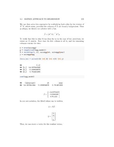
To verify that this is what R has done for us in the case of two predictors, we
create an matrix. Note that the first column is all 1s, and the remaining
columns contain the data.

n = nrow(autompg)
p = length(coef(mpg_model))
X = cbind(rep(1, n), autompg$wt, autompg$year)
y = autompg$mpg

(beta_hat = solve(t(X) %*% X) %*% t(X) %*% y)

## [,1]
## [1,] -14.637641945
## [2,] -0.006634876
## [3,] 0.761401955

coef(mpg_model)

## (Intercept) wt year
## -14.637641945 -0.006634876 0.761401955

−14.6376419
̂
= ⎡ −0.0066349 ⎤
⎥
⎢
⎣ 0.761402 ⎦
In our new notation, the fitted values can be written

̂ = . ̂

̂
1
⎡ ̂ ⎤
̂ = ⎢ 2 ⎥
⎢ ⋮ ⎥
⎣ ̂ ⎦

Then, we can create a vector for the residual values,