Page 172 - Applied Statistics with R

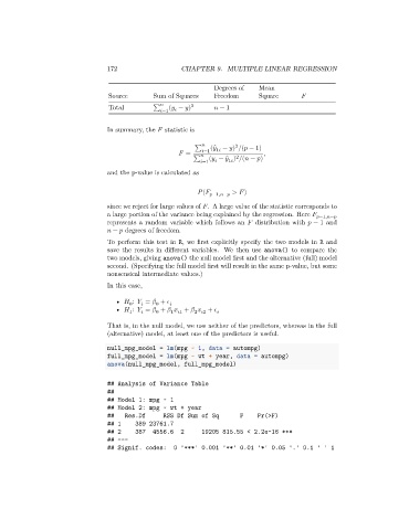
172 CHAPTER 9. MULTIPLE LINEAR REGRESSION

Degrees of Mean
Source Sum of Squares Freedom Square
2

Total ∑ ( − ̄) − 1
=1
In summary, the statistic is

2

∑ ( ̂ − ̄) /( − 1)
= =1 1 ,
2
∑ ( − ̂ ) /( − )

=1 1
and the p-value is calculated as
( −1, − > )
since we reject for large values of . A large value of the statistic corresponds to
a large portion of the variance being explained by the regression. Here −1, −
represents a random variable which follows an distribution with − 1 and
− degrees of freedom.

To perform this test in R, we first explicitly specify the two models in R and
save the results in different variables. We then use anova() to compare the
two models, giving anova() the null model first and the alternative (full) model
second. (Specifying the full model first will result in the same p-value, but some
nonsensical intermediate values.)

In this case,

• : = +

0
0
• : = + + +
1 1
2 2
0

1
That is, in the null model, we use neither of the predictors, whereas in the full
(alternative) model, at least one of the predictors is useful.
null_mpg_model = lm(mpg ~ 1, data = autompg)
full_mpg_model = lm(mpg ~ wt + year, data = autompg)
anova(null_mpg_model, full_mpg_model)
## Analysis of Variance Table
##
## Model 1: mpg ~ 1
## Model 2: mpg ~ wt + year
## Res.Df RSS Df Sum of Sq F Pr(>F)
## 1 389 23761.7
## 2 387 4556.6 2 19205 815.55 < 2.2e-16 ***
## ---
## Signif. codes: 0 '***' 0.001 '**' 0.01 '*' 0.05 '.' 0.1 ' ' 1