Page 167 - Applied Statistics with R

9.2. SAMPLING DISTRIBUTION 167

R then reports the estimate ̂( ) (fit) for each, as well as the lower (lwr) and
0
upper (upr) bounds for the interval at a desired level (99%).
A word of caution here: one of these estimates is good while one is suspect.

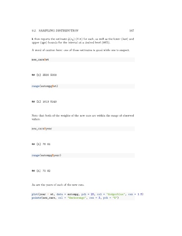
new_cars$wt

## [1] 3500 5000

range(autompg$wt)

## [1] 1613 5140

Note that both of the weights of the new cars are within the range of observed
values.

new_cars$year

## [1] 76 81

range(autompg$year)

## [1] 70 82

As are the years of each of the new cars.

plot(year ~ wt, data = autompg, pch = 20, col = "dodgerblue", cex = 1.5)
points(new_cars, col = "darkorange", cex = 3, pch = "X")