Page 169 - Applied Statistics with R

9.2. SAMPLING DISTRIBUTION 169

−14.6376419
⊤ ̂
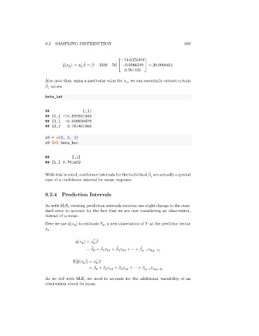
̂ ( ) = = [1 3500 76] ⎡ −0.0066349 ⎤ = 20.0068411
⎥
⎢
0
0
⎣ 0.761402 ⎦
Also note that, using a particular value for , we can essentially extract certain
0
̂
values.

beta_hat
## [,1]
## [1,] -14.637641945
## [2,] -0.006634876
## [3,] 0.761401955

x0 = c(0, 0, 1)
x0 %*% beta_hat

## [,1]
## [1,] 0.761402

̂
With this in mind, confidence intervals for the individual are actually a special

case of a confidence interval for mean response.

9.2.4 Prediction Intervals

As with SLR, creating prediction intervals involves one slight change to the stan-
dard error to account for the fact that we are now considering an observation,
instead of a mean.
Here we use ̂( ) to estimate , a new observation of at the predictor vector

0
0
.
0
⊤ ̂
̂ ( ) =
0
0
̂
̂
̂
̂
= + + + ⋯ + −1 0( −1)

2 02
0
1 01
⊤

E[ ̂( )] =
0
0
= + + + ⋯ + −1 0( −1)

1 01
2 02
0
As we did with SLR, we need to account for the additional variability of an
observation about its mean.