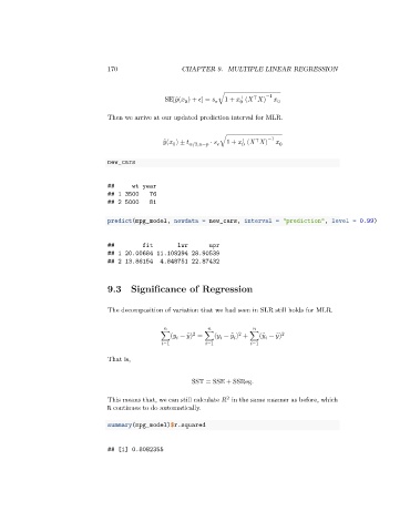
Page 170 - Applied Statistics with R

170 CHAPTER 9. MULTIPLE LINEAR REGRESSION

⊤
⊤
SE[ ̂( ) + ] = √ 1 + ( ) −1 0

0
0
Then we arrive at our updated prediction interval for MLR.
⊤
̂ ( ) ± /2, − ⋅ √ 1 + ( ) −1 0
⊤
0
0
new_cars

## wt year
## 1 3500 76
## 2 5000 81

predict(mpg_model, newdata = new_cars, interval = "prediction", level = 0.99)

## fit lwr upr
## 1 20.00684 11.108294 28.90539
## 2 13.86154 4.848751 22.87432

9.3 Significance of Regression

The decomposition of variation that we had seen in SLR still holds for MLR.

2
2

∑( − ̄) = ∑( − ̂ ) + ∑( ̂ − ̄) 2

=1 =1 =1
That is,
SST = SSE + SSReg.
2
This means that, we can still calculate in the same manner as before, which
R continues to do automatically.
summary(mpg_model)$r.squared

## [1] 0.8082355