Page 250 - Applied Statistics with R

250 CHAPTER 12. ANALYSIS OF VARIANCE

∑ = 0 ∑ = 0.

and

( ) 1 + ( ) 2 + ( ) 3 = 0( ) + ( ) + ( ) + ( ) 4 = 0
3
2
1
for any or .
Here,

• = 1, 2, … where is the number of levels of factor .
• = 1, 2, … where is the number of levels of factor .
• = 1, 2, … where is the number of replicates per group.

Here, we can think of a group as a combination of a level from each of the
factors. So for example, one group will receive level 2 of factor and level 3
of factor . The number of replicates is the number of subjects in each group.
Here 135 would be the measurement for the fifth member (replicate) of the
group for level 1 of factor and level 3 of factor .
We call this setup an × factorial design with replicates. (Our current
notation only allows for equal replicates in each group. It isn’t difficult to
allow for different replicates for different groups, but we’ll proceed using equal
replicates per group, which if possible, is desirable.)

• measures the effect of level of factor . We call these the main

effects of factor .
• measures the effect of level of factor . We call these the main

effects of factor .
• ( ) is a single parameter. We use to note that this parameter
measures the interaction between the two main effects.

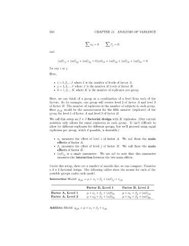
Under this setup, there are a number of models that we can compare. Consider
a 2 × 2 factorial design. The following tables show the means for each of the
possible groups under each model.
Interaction Model: = + + + ( ) +

Factor B, Level 1 Factor B, Level 2
Factor A, Level 1 + + + ( ) 11 + + + ( ) 12
2
1
1
1
Factor A, Level 2 + + + ( ) 21 + + + ( ) 22
2
2
2
1
Additive Model: = + + +