Page 264 - Applied Statistics with R

264 CHAPTER 13. MODEL DIAGNOSTICS

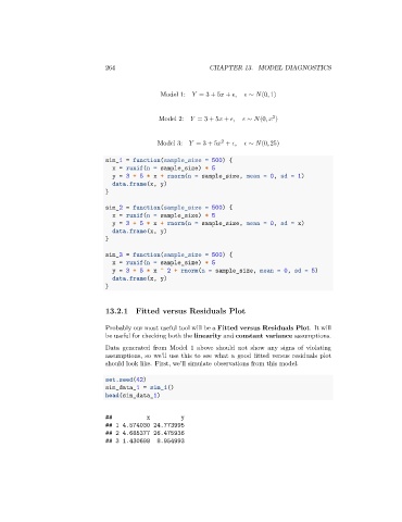
Model 1: = 3 + 5 + , ∼ (0, 1)

2
Model 2: = 3 + 5 + , ∼ (0, )

2
Model 3: = 3 + 5 + , ∼ (0, 25)

sim_1 = function(sample_size = 500) {
x = runif(n = sample_size) * 5
y = 3 + 5 * x + rnorm(n = sample_size, mean = 0, sd = 1)
data.frame(x, y)
}

sim_2 = function(sample_size = 500) {
x = runif(n = sample_size) * 5
y = 3 + 5 * x + rnorm(n = sample_size, mean = 0, sd = x)
data.frame(x, y)
}

sim_3 = function(sample_size = 500) {
x = runif(n = sample_size) * 5
y = 3 + 5 * x ^ 2 + rnorm(n = sample_size, mean = 0, sd = 5)
data.frame(x, y)
}

13.2.1 Fitted versus Residuals Plot

Probably our most useful tool will be a Fitted versus Residuals Plot. It will
be useful for checking both the linearity and constant variance assumptions.
Data generated from Model 1 above should not show any signs of violating
assumptions, so we’ll use this to see what a good fitted versus residuals plot
should look like. First, we’ll simulate observations from this model.

set.seed(42)
sim_data_1 = sim_1()
head(sim_data_1)

## x y
## 1 4.574030 24.773995
## 2 4.685377 26.475936
## 3 1.430698 8.954993