Page 268 - Applied Statistics with R

268 CHAPTER 13. MODEL DIAGNOSTICS

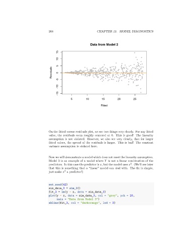
Data from Model 2

15

10

5
Residuals 0

-5

-10
-15

5 10 15 20 25

Fitted

On the fitted versus residuals plot, we see two things very clearly. For any fitted
value, the residuals seem roughly centered at 0. This is good! The linearity
assumption is not violated. However, we also see very clearly, that for larger
fitted values, the spread of the residuals is larger. This is bad! The constant
variance assumption is violated here.

Now we will demonstrate a model which does not meet the linearity assumption.
Model 3 is an example of a model where is not a linear combination of the
2
predictors. In this case the predictor is , but the model uses . (We’ll see later
that this is something that a “linear” model can deal with. The fix is simple,
2
just make a predictor!)

set.seed(42)
sim_data_3 = sim_3()
fit_3 = lm(y ~ x, data = sim_data_3)
plot(y ~ x, data = sim_data_3, col = "grey", pch = 20,
main = "Data from Model 3")
abline(fit_3, col = "darkorange", lwd = 3)