Page 265 - Applied Statistics with R

13.2. CHECKING ASSUMPTIONS 265

## 4 4.152238 23.951210
## 5 3.208728 20.341344
## 6 2.595480 14.943525

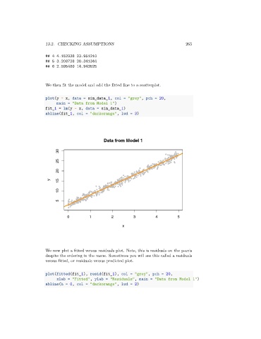
We then fit the model and add the fitted line to a scatterplot.

plot(y ~ x, data = sim_data_1, col = "grey", pch = 20,
main = "Data from Model 1")
fit_1 = lm(y ~ x, data = sim_data_1)
abline(fit_1, col = "darkorange", lwd = 3)

Data from Model 1

30
25

20

y
15
10

5

0 1 2 3 4 5

x

We now plot a fitted versus residuals plot. Note, this is residuals on the -axis
despite the ordering in the name. Sometimes you will see this called a residuals
versus fitted, or residuals versus predicted plot.

plot(fitted(fit_1), resid(fit_1), col = "grey", pch = 20,
xlab = "Fitted", ylab = "Residuals", main = "Data from Model 1")
abline(h = 0, col = "darkorange", lwd = 2)