Page 267 - Applied Statistics with R
P. 267

13.2. CHECKING ASSUMPTIONS                                        267
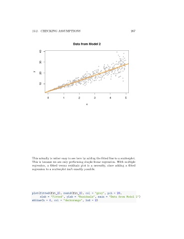


                                                  Data from Model 2

                             40


                             30


                        y
                             20


                             10


                                 0         1         2          3         4         5

                                                          x


                      This actually is rather easy to see here by adding the fitted line to a scatterplot.
                      This is because we are only performing simple linear regression. With multiple
                      regression, a fitted versus residuals plot is a necessity, since adding a fitted
                      regression to a scatterplot isn’t exactly possible.


                      plot(fitted(fit_2), resid(fit_2), col = "grey", pch = 20,
                            xlab = "Fitted", ylab = "Residuals", main = "Data from Model 2")
                      abline(h = 0, col = "darkorange", lwd = 2)
   262   263   264   265   266   267   268   269   270   271   272