Page 266 - Applied Statistics with R

266 CHAPTER 13. MODEL DIAGNOSTICS

Data from Model 1

3

2
Residuals 1 0

-1

-2

-3
5 10 15 20 25

Fitted

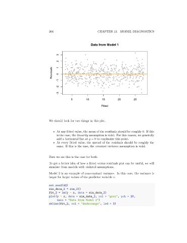
We should look for two things in this plot.

• At any fitted value, the mean of the residuals should be roughly 0. If this
is the case, the linearity assumption is valid. For this reason, we generally
add a horizontal line at = 0 to emphasize this point.
• At every fitted value, the spread of the residuals should be roughly the
same. If this is the case, the constant variance assumption is valid.

Here we see this is the case for both.

To get a better idea of how a fitted versus residuals plot can be useful, we will
simulate from models with violated assumptions.

Model 2 is an example of non-constant variance. In this case, the variance is
larger for larger values of the predictor variable .

set.seed(42)
sim_data_2 = sim_2()
fit_2 = lm(y ~ x, data = sim_data_2)
plot(y ~ x, data = sim_data_2, col = "grey", pch = 20,
main = "Data from Model 2")
abline(fit_2, col = "darkorange", lwd = 3)