Page 292 - Applied Statistics with R

292 CHAPTER 13. MODEL DIAGNOSTICS

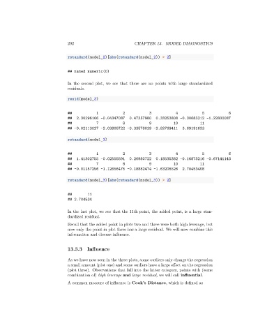
rstandard(model_2)[abs(rstandard(model_2)) > 2]

## named numeric(0)

In the second plot, we see that there are no points with large standardized
residuals.

resid(model_3)

## 1 2 3 4 5 6
## 2.30296166 -0.04347087 0.47357980 0.33253808 -0.30683212 -1.22800087
## 7 8 9 10 11
## -0.02113027 -2.03808722 -0.33578039 -2.82769411 3.69191633

rstandard(model_3)

## 1 2 3 4 5 6
## 1.41302755 -0.02555591 0.26980722 0.18535382 -0.16873216 -0.67141143
## 7 8 9 10 11
## -0.01157256 -1.12656475 -0.18882474 -1.63206526 2.70453408

rstandard(model_3)[abs(rstandard(model_3)) > 2]

## 11
## 2.704534

In the last plot, we see that the 11th point, the added point, is a large stan-
dardized residual.

Recall that the added point in plots two and three were both high leverage, but
now only the point in plot three has a large residual. We will now combine this
information and discuss influence.

13.3.3 Influence

As we have now seen in the three plots, some outliers only change the regression
a small amount (plot one) and some outliers have a large effect on the regression
(plot three). Observations that fall into the latter category, points with (some
combination of) high leverage and large residual, we will call influential.
A common measure of influence is Cook’s Distance, which is defined as