Page 320 - Applied Statistics with R

320 CHAPTER 14. TRANSFORMATIONS

## $ acc : num 12 11.5 11 12 10.5 10 9 8.5 10 8.5 ...
## $ year : int 70 70 70 70 70 70 70 70 70 70 ...
## $ origin : int 1 1 1 1 1 1 1 1 1 1 ...
## $ domestic: num 1 1 1 1 1 1 1 1 1 1 ...

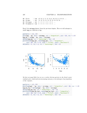
Recall the autompg dataset from the previous chapter. Here we will attempt to
model mpg as a function of hp.

par(mfrow = c(1, 2))
plot(mpg ~ hp, data = autompg, col = "dodgerblue", pch = 20, cex = 1.5)
mpg_hp = lm(mpg ~ hp, data = autompg)
abline(mpg_hp, col = "darkorange", lwd = 2)
plot(fitted(mpg_hp), resid(mpg_hp), col = "dodgerblue",
pch = 20, cex = 1.5, xlab = "Fitted", ylab = "Residuals")
abline(h = 0, lty = 2, col = "darkorange", lwd = 2)

15
40 10

mpg 30 Residuals 5 0
20
-10
10

50 100 150 200 5 10 15 20 25 30
hp Fitted

We first attempt SLR, but we see a rather obvious pattern in the fitted versus
residuals plot, which includes increasing variance, so we attempt a log transform
of the response.

par(mfrow = c(1, 2))
plot(log(mpg) ~ hp, data = autompg, col = "dodgerblue", pch = 20, cex = 1.5)
mpg_hp_log = lm(log(mpg) ~ hp, data = autompg)
abline(mpg_hp_log, col = "darkorange", lwd = 2)
plot(fitted(mpg_hp_log), resid(mpg_hp_log), col = "dodgerblue",
pch = 20, cex = 1.5, xlab = "Fitted", ylab = "Residuals")
abline(h = 0, lty = 2, col = "darkorange", lwd = 2)