Page 321 - Applied Statistics with R

14.2. PREDICTOR TRANSFORMATION 321

0.6
3.5 0.2
log(mpg) 3.0 Residuals -0.2

2.5
-0.6

50 100 150 200 2.2 2.4 2.6 2.8 3.0 3.2 3.4
hp Fitted

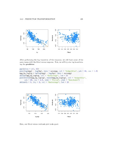
After performing the log transform of the response, we still have some of the
same issues with the fitted versus response. Now, we will try also log transform-
ing the predictor.

par(mfrow = c(1, 2))
plot(log(mpg) ~ log(hp), data = autompg, col = "dodgerblue", pch = 20, cex = 1.5)
mpg_hp_loglog = lm(log(mpg) ~ log(hp), data = autompg)
abline(mpg_hp_loglog, col = "darkorange", lwd = 2)
plot(fitted(mpg_hp_loglog), resid(mpg_hp_loglog), col = "dodgerblue",
pch = 20, cex = 1.5, xlab = "Fitted", ylab = "Residuals")
abline(h = 0, lty = 2, col = "darkorange", lwd = 2)

0.6
3.5 0.2
log(mpg) 3.0 Residuals -0.2

2.5
-0.6

4.0 4.5 5.0 5.5 2.4 2.6 2.8 3.0 3.2 3.4 3.6
log(hp) Fitted

Here, our fitted versus residuals plot looks good.