Page 325 - Applied Statistics with R

14.2. PREDICTOR TRANSFORMATION 325

## [,1] [,2] [,3]
## [1,] 21.00 120.70 1107.95
## [2,] 120.70 1107.95 12385.86
## [3,] 1107.95 12385.86 151369.12

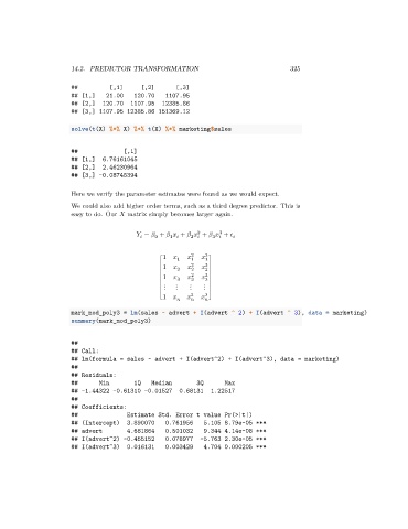
solve(t(X) %*% X) %*% t(X) %*% marketing$sales

## [,1]
## [1,] 6.76161045
## [2,] 2.46230964
## [3,] -0.08745394

Here we verify the parameter estimates were found as we would expect.
We could also add higher order terms, such as a third degree predictor. This is
easy to do. Our matrix simply becomes larger again.

2
3
= + + + +
2
3

0
1
1 1 2 1 3 1
⎡ 2 3 ⎤
⎢ 1 2 2 2⎥
⎢ 1 2 3 ⎥
⎢ 3 3 3 ⎥
⎢ ⋮ ⋮ ⋮ ⋮ ⎥
3
⎣1 2 ⎦

mark_mod_poly3 = lm(sales ~ advert + I(advert ^ 2) + I(advert ^ 3), data = marketing)
summary(mark_mod_poly3)

##
## Call:
## lm(formula = sales ~ advert + I(advert^2) + I(advert^3), data = marketing)
##
## Residuals:
## Min 1Q Median 3Q Max
## -1.44322 -0.61310 -0.01527 0.68131 1.22517
##
## Coefficients:
## Estimate Std. Error t value Pr(>|t|)
## (Intercept) 3.890070 0.761956 5.105 8.79e-05 ***
## advert 4.681864 0.501032 9.344 4.14e-08 ***
## I(advert^2) -0.455152 0.078977 -5.763 2.30e-05 ***
## I(advert^3) 0.016131 0.003429 4.704 0.000205 ***