Page 324 - Applied Statistics with R

324 CHAPTER 14. TRANSFORMATIONS

## Coefficients:
## Estimate Std. Error t value Pr(>|t|)
## (Intercept) 9.4502 0.6806 13.88 2.13e-11 ***
## advert 1.1918 0.0937 12.72 9.65e-11 ***
## ---
## Signif. codes: 0 '***' 0.001 '**' 0.01 '*' 0.05 '.' 0.1 ' ' 1
##
## Residual standard error: 1.907 on 19 degrees of freedom
## Multiple R-squared: 0.8949, Adjusted R-squared: 0.8894
## F-statistic: 161.8 on 1 and 19 DF, p-value: 9.646e-11

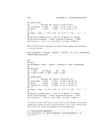
While the SLR model is significant, the fitted versus residuals plot would have
a very clear pattern.

mark_mod_poly2 = lm(sales ~ advert + I(advert ^ 2), data = marketing)
summary(mark_mod_poly2)

##
## Call:
## lm(formula = sales ~ advert + I(advert^2), data = marketing)
##
## Residuals:
## Min 1Q Median 3Q Max
## -1.9175 -0.8333 -0.1948 0.9292 2.1385
##
## Coefficients:
## Estimate Std. Error t value Pr(>|t|)
## (Intercept) 6.76161 0.67219 10.059 8.16e-09 ***
## advert 2.46231 0.24830 9.917 1.02e-08 ***
## I(advert^2) -0.08745 0.01658 -5.275 5.14e-05 ***
## ---
## Signif. codes: 0 '***' 0.001 '**' 0.01 '*' 0.05 '.' 0.1 ' ' 1
##
## Residual standard error: 1.228 on 18 degrees of freedom
## Multiple R-squared: 0.9587, Adjusted R-squared: 0.9541
## F-statistic: 209 on 2 and 18 DF, p-value: 3.486e-13

To add the second order term we need to use the I() function in the model
specification around our newly created predictor. We see that with the first
order term in the model, the quadratic term is also significant.

n = length(marketing$advert)
X = cbind(rep(1, n), marketing$advert, marketing$advert ^ 2)
t(X) %*% X