Page 323 - Applied Statistics with R

14.2. PREDICTOR TRANSFORMATION 323

2
where ∼ (0, ) for = 1, 2, ⋯ 21.

The response is now a linear function of “two” variables which now allows
to be a non-linear function of the original single predictor . We consider
this a transformation, although we have actually in some sense added another
predictor.

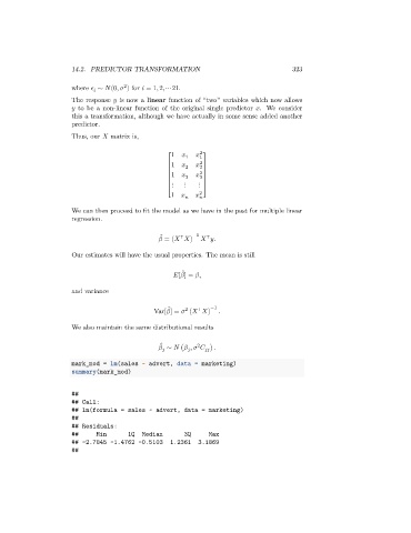
Thus, our matrix is,

1 1 2 1
⎡ 2 ⎤
⎢ 1 2 2⎥
⎢ 1 2 ⎥
⎢ 3 3 ⎥
⎢ ⋮ ⋮ ⋮ ⎥
2
⎣1 ⎦

We can then proceed to fit the model as we have in the past for multiple linear
regression.

̂
⊤
⊤
= ( ) −1 .
Our estimates will have the usual properties. The mean is still

̂
[ ] = ,

and variance

̂
⊤
2
Var[ ] = ( ) −1 .
We also maintain the same distributional results

̂
2
∼ ( , ) .

mark_mod = lm(sales ~ advert, data = marketing)
summary(mark_mod)
##
## Call:
## lm(formula = sales ~ advert, data = marketing)
##
## Residuals:
## Min 1Q Median 3Q Max
## -2.7845 -1.4762 -0.5103 1.2361 3.1869
##