Page 326 - Applied Statistics with R

326 CHAPTER 14. TRANSFORMATIONS

## ---
## Signif. codes: 0 '***' 0.001 '**' 0.01 '*' 0.05 '.' 0.1 ' ' 1
##
## Residual standard error: 0.8329 on 17 degrees of freedom
## Multiple R-squared: 0.9821, Adjusted R-squared: 0.9789
## F-statistic: 310.2 on 3 and 17 DF, p-value: 4.892e-15

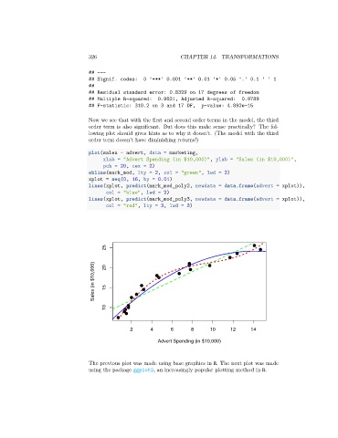
Now we see that with the first and second order terms in the model, the third
order term is also significant. But does this make sense practically? The fol-
lowing plot should gives hints as to why it doesn’t. (The model with the third
order term doesn’t have diminishing returns!)

plot(sales ~ advert, data = marketing,
xlab = "Advert Spending (in $10,000)", ylab = "Sales (in $10,000)",
pch = 20, cex = 2)
abline(mark_mod, lty = 2, col = "green", lwd = 2)
xplot = seq(0, 16, by = 0.01)
lines(xplot, predict(mark_mod_poly2, newdata = data.frame(advert = xplot)),
col = "blue", lwd = 2)
lines(xplot, predict(mark_mod_poly3, newdata = data.frame(advert = xplot)),
col = "red", lty = 3, lwd = 3)

25

Sales (in $10,000) 20 15

10

2 4 6 8 10 12 14

Advert Spending (in $10,000)

The previous plot was made using base graphics in R. The next plot was made
using the package ggplot2, an increasingly popular plotting method in R.