Page 374 - Applied Statistics with R

374 CHAPTER 15. COLLINEARITY

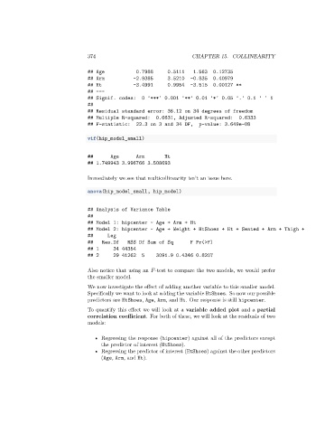
## Age 0.7988 0.5111 1.563 0.12735
## Arm -2.9385 3.5210 -0.835 0.40979
## Ht -3.4991 0.9954 -3.515 0.00127 **
## ---
## Signif. codes: 0 '***' 0.001 '**' 0.01 '*' 0.05 '.' 0.1 ' ' 1
##
## Residual standard error: 36.12 on 34 degrees of freedom
## Multiple R-squared: 0.6631, Adjusted R-squared: 0.6333
## F-statistic: 22.3 on 3 and 34 DF, p-value: 3.649e-08

vif(hip_model_small)

## Age Arm Ht
## 1.749943 3.996766 3.508693

Immediately we see that multicollinearity isn’t an issue here.

anova(hip_model_small, hip_model)

## Analysis of Variance Table
##
## Model 1: hipcenter ~ Age + Arm + Ht
## Model 2: hipcenter ~ Age + Weight + HtShoes + Ht + Seated + Arm + Thigh +
## Leg
## Res.Df RSS Df Sum of Sq F Pr(>F)
## 1 34 44354
## 2 29 41262 5 3091.9 0.4346 0.8207

Also notice that using an -test to compare the two models, we would prefer
the smaller model.

We now investigate the effect of adding another variable to this smaller model.
Specifically we want to look at adding the variable HtShoes. So now our possible
predictors are HtShoes, Age, Arm, and Ht. Our response is still hipcenter.
To quantify this effect we will look at a variable added plot and a partial
correlation coefficient. For both of these, we will look at the residuals of two
models:

• Regressing the response (hipcenter) against all of the predictors except
the predictor of interest (HtShoes).
• Regressing the predictor of interest (HtShoes) against the other predictors
(Age, Arm, and Ht).