Page 428 - Applied Statistics with R

428 CHAPTER 17. LOGISTIC REGRESSION

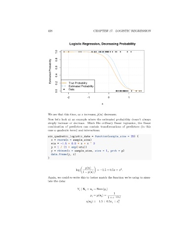
Logistic Regression, Decreasing Probability

1.0 0.8

Estimated Probability 0.6 0.4

0.2
True Probability
Estimated Probability
0.0 Data

-2 -1 0 1

x

We see that this time, as increases, ̂(x) decreases.
Now let’s look at an example where the estimated probability doesn’t always
simply increase or decrease. Much like ordinary linear regression, the linear
combination of predictors can contain transformations of predictors (in this
case a quadratic term) and interactions.
sim_quadratic_logistic_data = function(sample_size = 25) {
x = rnorm(n = sample_size)
eta = -1.5 + 0.5 * x + x ^ 2
p = 1 / (1 + exp(-eta))
y = rbinom(n = sample_size, size = 1, prob = p)
data.frame(y, x)
}

(x)
2
log ( ) = −1.5 + 0.5 + .
1 − (x)
Again, we could re-write this to better match the function we’re using to simu-
late the data:

∣ X = x ∼ Bern( )
i

i

1
= (x ) =

i
1 + − (x i )
(x ) = −1.5 + 0.5 + 2
i