Page 424 - Applied Statistics with R

424 CHAPTER 17. LOGISTIC REGRESSION

After simulating a dataset, we’ll then fit both ordinary linear regression and
logistic regression. Notice that currently the responses variable y is a numeric
variable that only takes values 0 and 1. Later we’ll see that we can also fit
logistic regression when the response is a factor variable with only two levels.
(Generally, having a factor response is preferred, but having a dummy response
allows use to make the comparison to using ordinary linear regression.)

# ordinary linear regression
fit_lm = lm(y ~ x, data = example_data)
# logistic regression
fit_glm = glm(y ~ x, data = example_data, family = binomial)

Notice that the syntax is extremely similar. What’s changed?

• lm() has become glm()
• We’ve added family = binomial argument

In a lot of ways, lm() is just a more specific version of glm(). For example

glm(y ~ x, data = example_data)

would actually fit the ordinary linear regression that we have seen in the past.
By default, glm() uses family = gaussian argument. That is, we’re fitting
a GLM with a normally distributed response and the identity function as the
link.
The family argument to glm() actually specifies both the distribution and the
link function. If not made explicit, the link function is chosen to be the canon-
ical link function, which is essentially the most mathematical convenient link
function. See ?glm and ?family for details. For example, the following code
explicitly specifies the link function which was previously used by default.

# more detailed call to glm for logistic regression
fit_glm = glm(y ~ x, data = example_data, family = binomial(link = "logit"))

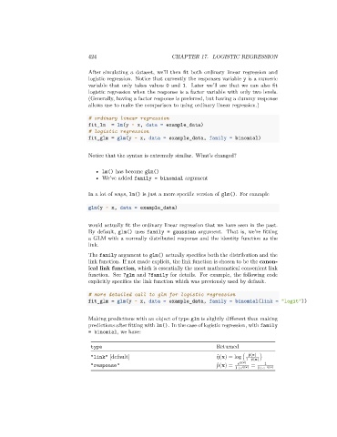
Making predictions with an object of type glm is slightly different than making
predictions after fitting with lm(). In the case of logistic regression, with family
= binomial, we have:

type Returned
̂ (x)
"link" [default] ̂ (x) = log ( 1− ̂ (x) )
"response" ̂ (x) = ̂ (x) ̂ (x) = 1
1+ 1+ − ̂ (x)