Page 429 - Applied Statistics with R

17.3. WORKING WITH LOGISTIC REGRESSION 429

set.seed(42)
example_data = sim_quadratic_logistic_data(sample_size = 50)

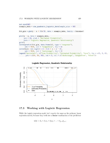
fit_glm = glm(y ~ x + I(x^2), data = example_data, family = binomial)

plot(y ~ x, data = example_data,
pch = 20, ylab = "Estimated Probability",
main = "Logistic Regression, Quadratic Relationship")
grid()
curve(predict(fit_glm, data.frame(x), type = "response"),
add = TRUE, col = "dodgerblue", lty = 2)
curve(boot::inv.logit(-1.5 + 0.5 * x + x ^ 2),
add = TRUE, col = "darkorange", lty = 1)
legend("bottomleft", c("True Probability", "Estimated Probability", "Data"), lty = c(1, 2, 0),
pch = c(NA, NA, 20), lwd = 2, col = c("darkorange", "dodgerblue", "black"))

Logistic Regression, Quadratic Relationship

1.0 0.8

Estimated Probability 0.6 0.4

0.2
True Probability
Estimated Probability
0.0 Data

-2 -1 0 1 2
x

17.3 Working with Logistic Regression

While the logistic regression model isn’t exactly the same as the ordinary linear
regression model, because they both use a linear combination of the predictors

(x) = + + + … + −1 −1
2 2
0
1 1