Page 437 - Applied Statistics with R
P. 437

17.3. WORKING WITH LOGISTIC REGRESSION                            437


                      new_obs = data.frame(
                        sbp = 148.0,
                        tobacco = 5,
                        ldl = 12,
                        adiposity = 31.23,
                        famhist = "Present",
                        typea = 47,
                        obesity = 28.50,
                        alcohol = 23.89,
                        age = 60
                      )


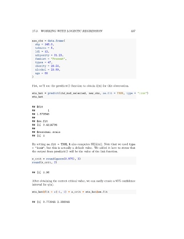
                      Fist, we’ll use the predict() function to obtain ̂(x) for this observation.
                                                                   
                      eta_hat = predict(chd_mod_selected, new_obs, se.fit = TRUE, type = "link")
                      eta_hat


                      ## $fit
                      ##         1
                      ## 1.579545
                      ##
                      ## $se.fit
                      ## [1] 0.4114796
                      ##
                      ## $residual.scale
                      ## [1] 1

                      By setting se.fit = TRUE, R also computes SE[ ̂(x)]. Note that we used type
                                                                  
                      = "link", but this is actually a default value. We added it here to stress that
                      the output from predict() will be the value of the link function.

                      z_crit = round(qnorm(0.975), 2)
                      round(z_crit, 2)


                      ## [1] 1.96

                      After obtaining the correct critical value, we can easily create a 95% confidence
                      interval for   (x).

                      eta_hat$fit + c(-1, 1) * z_crit * eta_hat$se.fit


                      ## [1] 0.773045 2.386045
   432   433   434   435   436   437   438   439   440   441   442