Page 438 - Applied Statistics with R

438 CHAPTER 17. LOGISTIC REGRESSION

Now we simply need to apply the correct transformation to make this a confi-
dence interval for (x), the probability of coronary heart disease for this observa-
tion. Note that the boot package contains functions logit() and inv.logit()
which are the logit and inverse logit transformations, respectively.

boot::inv.logit(eta_hat$fit + c(-1, 1) * z_crit * eta_hat$se.fit)

## [1] 0.6841792 0.9157570

Notice, as we would expect, the bounds of this interval are both between 0 and
1. Also, since both bounds of the interval for (x) are positive, both bounds of
the interval for (x) are greater than 0.5.

17.3.7 Formula Syntax

Without really thinking about it, we’ve been using our previous knowledge of
R’s model formula syntax to fit logistic regression.

17.3.7.1 Interactions

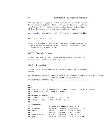
Let’s add an interaction between LDL and family history for the model we
selected.

chd_mod_interaction = glm(chd ~ alcohol + ldl + famhist + typea + age + ldl:famhist,
data = SAheart, family = binomial)
summary(chd_mod_interaction)

##
## Call:
## glm(formula = chd ~ alcohol + ldl + famhist + typea + age + ldl:famhist,
## family = binomial, data = SAheart)
##
## Deviance Residuals:
## Min 1Q Median 3Q Max
## -1.9082 -0.8308 -0.4550 0.9286 2.5152
##
## Coefficients:
## Estimate Std. Error z value Pr(>|z|)
## (Intercept) -6.043472 0.937186 -6.449 1.13e-10 ***
## alcohol 0.003800 0.004332 0.877 0.38033
## ldl 0.035593 0.071448 0.498 0.61837
## famhistPresent -0.733836 0.618131 -1.187 0.23515
## typea 0.036253 0.012172 2.978 0.00290 **