Page 436 - Applied Statistics with R

436 CHAPTER 17. LOGISTIC REGRESSION

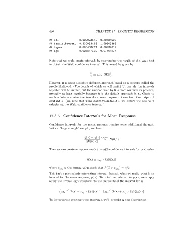
## ldl 0.022923610 0.30784590
## famhistPresent 0.330033483 1.49603366
## typea 0.006408724 0.06932612
## age 0.024847330 0.07764277

Note that we could create intervals by rearranging the results of the Wald test
to obtain the Wald confidence interval. This would be given by

̂
̂
± /2 ⋅ SE[ ].

However, R is using a slightly different approach based on a concept called the
profile likelihood. (The details of which we will omit.) Ultimately the intervals
reported will be similar, but the method used by R is more common in practice,
probably at least partially because it is the default approach in R. Check to
see how intervals using the formula above compare to those from the output of
confint(). (Or, note that using confint.default() will return the results of
calculating the Wald confidence interval.)

17.3.6 Confidence Intervals for Mean Response

Confidence intervals for the mean response require some additional thought.
With a “large enough” sample, we have

̂ (x) − (x) approx (0, 1)
∼
SE[ ̂(x)]

Then we can create an approximate (1− )% confidence intervals for (x) using

̂ (x) ± /2 ⋅ SE[ ̂(x)]

where /2 is the critical value such that ( > /2 ) = /2.
This isn’t a particularly interesting interval. Instead, what we really want is an
interval for the mean response, (x). To obtain an interval for (x), we simply
apply the inverse logit transform to the endpoints of the interval for .

−1
−1

(logit ( ̂(x) − /2 ⋅ SE[ ̂(x)]), logit ( ̂(x) + /2 ⋅ SE[ ̂(x)]))
To demonstrate creating these intervals, we’ll consider a new observation.