Page 434 - Applied Statistics with R

434 CHAPTER 17. LOGISTIC REGRESSION

we use the summary() function as we have done so many times before. Like the
-test for ordinary linear regression, this returns the estimate of the parameter,
its standard error, the relevant test statistic ( ), and its p-value. Here we have
an incredibly low p-value, so we reject the null hypothesis. The ldl variable
appears to be a significant predictor.
When fitting logistic regression, we can use the same formula syntax as ordinary
linear regression. So, to fit an additive model using all available predictors, we
use:

chd_mod_additive = glm(chd ~ ., data = SAheart, family = binomial)

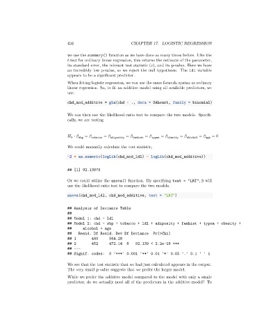
We can then use the likelihood-ratio test to compare the two models. Specifi-
cally, we are testing

∶ sbp = tobacco = adiposity = famhist = typea = obesity = alcohol = age = 0
0
We could manually calculate the test statistic,

-2 * as.numeric(logLik(chd_mod_ldl) - logLik(chd_mod_additive))

## [1] 92.13879

Or we could utilize the anova() function. By specifying test = "LRT", R will
use the likelihood-ratio test to compare the two models.

anova(chd_mod_ldl, chd_mod_additive, test = "LRT")

## Analysis of Deviance Table
##
## Model 1: chd ~ ldl
## Model 2: chd ~ sbp + tobacco + ldl + adiposity + famhist + typea + obesity +
## alcohol + age
## Resid. Df Resid. Dev Df Deviance Pr(>Chi)
## 1 460 564.28
## 2 452 472.14 8 92.139 < 2.2e-16 ***
## ---
## Signif. codes: 0 '***' 0.001 '**' 0.01 '*' 0.05 '.' 0.1 ' ' 1

We see that the test statistic that we had just calculated appears in the output.
The very small p-value suggests that we prefer the larger model.

While we prefer the additive model compared to the model with only a single
predictor, do we actually need all of the predictors in the additive model? To