Page 433 - Applied Statistics with R

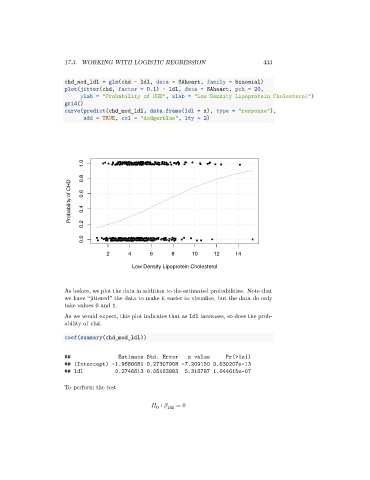
17.3. WORKING WITH LOGISTIC REGRESSION 433

chd_mod_ldl = glm(chd ~ ldl, data = SAheart, family = binomial)
plot(jitter(chd, factor = 0.1) ~ ldl, data = SAheart, pch = 20,
ylab = "Probability of CHD", xlab = "Low Density Lipoprotein Cholesterol")
grid()
curve(predict(chd_mod_ldl, data.frame(ldl = x), type = "response"),
add = TRUE, col = "dodgerblue", lty = 2)

1.0

0.8
Probability of CHD 0.6 0.4

0.2

0.0

2 4 6 8 10 12 14
Low Density Lipoprotein Cholesterol

As before, we plot the data in addition to the estimated probabilities. Note that
we have “jittered” the data to make it easier to visualize, but the data do only
take values 0 and 1.

As we would expect, this plot indicates that as ldl increases, so does the prob-
ability of chd.

coef(summary(chd_mod_ldl))

## Estimate Std. Error z value Pr(>|z|)
## (Intercept) -1.9686681 0.27307908 -7.209150 5.630207e-13
## ldl 0.2746613 0.05163983 5.318787 1.044615e-07

To perform the test

∶ ldl = 0
0