Page 148 - Python Data Science Handbook

Texas 2000 20851820
2010 25145561
dtype: int64
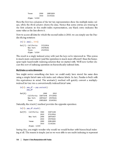
Here the first two columns of the Series representation show the multiple index val‐
ues, while the third column shows the data. Notice that some entries are missing in
the first column: in this multi-index representation, any blank entry indicates the
same value as the line above it.
Now to access all data for which the second index is 2010, we can simply use the Pan‐
das slicing notation:
In[7]: pop[:, 2010]
Out[7]: California 37253956
New York 19378102
Texas 25145561
dtype: int64
The result is a singly indexed array with just the keys we’re interested in. This syntax
is much more convenient (and the operation is much more efficient!) than the home-
spun tuple-based multi-indexing solution that we started with. We’ll now further dis‐
cuss this sort of indexing operation on hierarchically indexed data.

MultiIndex as extra dimension
You might notice something else here: we could easily have stored the same data
using a simple DataFrame with index and column labels. In fact, Pandas is built with
this equivalence in mind. The unstack() method will quickly convert a multiply-
indexed Series into a conventionally indexed DataFrame:

In[8]: pop_df = pop.unstack()
pop_df
Out[8]: 2000 2010
California 33871648 37253956
New York 18976457 19378102
Texas 20851820 25145561
Naturally, the stack() method provides the opposite operation:

In[9]: pop_df.stack()
Out[9]: California 2000 33871648
2010 37253956
New York 2000 18976457
2010 19378102
Texas 2000 20851820
2010 25145561
dtype: int64
Seeing this, you might wonder why would we would bother with hierarchical index‐
ing at all. The reason is simple: just as we were able to use multi-indexing to represent

130 | Chapter 3: Data Manipulation with Pandas