Page 215 - Python Data Science Handbook

financial data from a number of available sources, including Yahoo finance, Google
Finance, and others. Here we will load Google’s closing price history:

In[25]: from pandas_datareader import data
goog = data.DataReader('GOOG', start='2004', end='2016',
data_source='google')
goog.head()
Out[25]: Open High Low Close Volume
Date
2004-08-19 49.96 51.98 47.93 50.12 NaN
2004-08-20 50.69 54.49 50.20 54.10 NaN
2004-08-23 55.32 56.68 54.47 54.65 NaN
2004-08-24 55.56 55.74 51.73 52.38 NaN
2004-08-25 52.43 53.95 51.89 52.95 NaN
For simplicity, we’ll use just the closing price:

In[26]: goog = goog['Close']
We can visualize this using the plot() method, after the normal Matplotlib setup
boilerplate (Figure 3-5):

In[27]: %matplotlib inline
import matplotlib.pyplot as plt
import seaborn; seaborn.set()
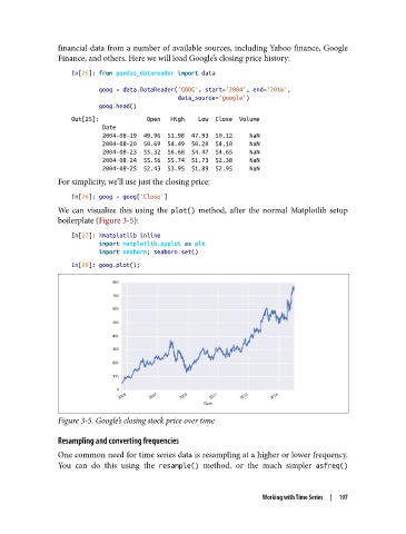
In[28]: goog.plot();

Figure 3-5. Google’s closing stock price over time

Resampling and converting frequencies

One common need for time series data is resampling at a higher or lower frequency.
You can do this using the resample() method, or the much simpler asfreq()

Working with Time Series | 197