Page 408 - Python Data Science Handbook

• When the naive assumptions actually match the data (very rare in practice)
• For very well-separated categories, when model complexity is less important
• For very high-dimensional data, when model complexity is less important

The last two points seem distinct, but they actually are related: as the dimension of a
dataset grows, it is much less likely for any two points to be found close together
(after all, they must be close in every single dimension to be close overall). This means
that clusters in high dimensions tend to be more separated, on average, than clusters
in low dimensions, assuming the new dimensions actually add information. For this
reason, simplistic classifiers like naive Bayes tend to work as well or better than more
complicated classifiers as the dimensionality grows: once you have enough data, even
a simple model can be very powerful.

In Depth: Linear Regression

Just as naive Bayes (discussed earlier in “In Depth: Naive Bayes Classification” on
page 382) is a good starting point for classification tasks, linear regression models are
a good starting point for regression tasks. Such models are popular because they can
be fit very quickly, and are very interpretable. You are probably familiar with the sim‐
plest form of a linear regression model (i.e., fitting a straight line to data), but such
models can be extended to model more complicated data behavior.

In this section we will start with a quick intuitive walk-through of the mathematics
behind this well-known problem, before moving on to see how linear models can be
generalized to account for more complicated patterns in data. We begin with the stan‐
dard imports:

In[1]: %matplotlib inline
import matplotlib.pyplot as plt
import seaborn as sns; sns.set()
import numpy as np
Simple Linear Regression

We will start with the most familiar linear regression, a straight-line fit to data. A
straight-line fit is a model of the form y = ax + b where a is commonly known as the
slope, and b is commonly known as the intercept.
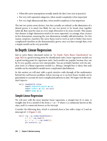
Consider the following data, which is scattered about a line with a slope of 2 and an
intercept of –5 (Figure 5-42):
In[2]: rng = np.random.RandomState(1)
x = 10 * rng.rand(50)
y = 2 * x - 5 + rng.randn(50)
plt.scatter(x, y);

390 | Chapter 5: Machine Learning