Page 404 - Python Data Science Handbook

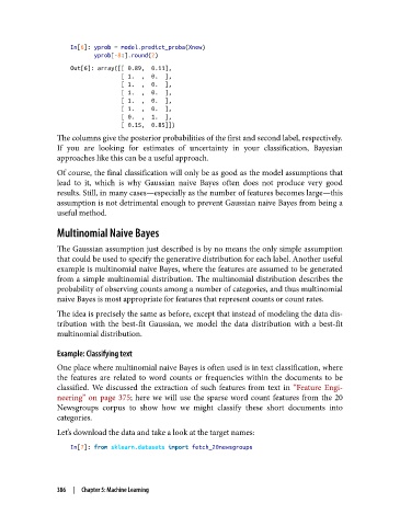
In[6]: yprob = model.predict_proba(Xnew)
yprob[-8:].round(2)
Out[6]: array([[ 0.89, 0.11],
[ 1. , 0. ],
[ 1. , 0. ],
[ 1. , 0. ],
[ 1. , 0. ],
[ 1. , 0. ],
[ 0. , 1. ],
[ 0.15, 0.85]])
The columns give the posterior probabilities of the first and second label, respectively.
If you are looking for estimates of uncertainty in your classification, Bayesian
approaches like this can be a useful approach.
Of course, the final classification will only be as good as the model assumptions that
lead to it, which is why Gaussian naive Bayes often does not produce very good
results. Still, in many cases—especially as the number of features becomes large—this
assumption is not detrimental enough to prevent Gaussian naive Bayes from being a
useful method.

Multinomial Naive Bayes

The Gaussian assumption just described is by no means the only simple assumption
that could be used to specify the generative distribution for each label. Another useful
example is multinomial naive Bayes, where the features are assumed to be generated
from a simple multinomial distribution. The multinomial distribution describes the
probability of observing counts among a number of categories, and thus multinomial
naive Bayes is most appropriate for features that represent counts or count rates.
The idea is precisely the same as before, except that instead of modeling the data dis‐
tribution with the best-fit Gaussian, we model the data distribution with a best-fit
multinomial distribution.

Example: Classifying text
One place where multinomial naive Bayes is often used is in text classification, where
the features are related to word counts or frequencies within the documents to be
classified. We discussed the extraction of such features from text in “Feature Engi‐
neering” on page 375; here we will use the sparse word count features from the 20
Newsgroups corpus to show how we might classify these short documents into
categories.
Let’s download the data and take a look at the target names:

In[7]: from sklearn.datasets import fetch_20newsgroups

386 | Chapter 5: Machine Learning