Page 410 - Python Data Science Handbook

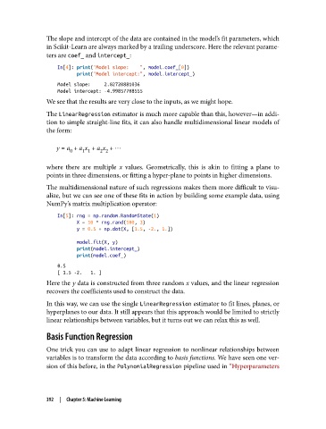
The slope and intercept of the data are contained in the model’s fit parameters, which
in Scikit-Learn are always marked by a trailing underscore. Here the relevant parame‐
ters are coef_ and intercept_:
In[4]: print("Model slope: ", model.coef_[0])
print("Model intercept:", model.intercept_)
Model slope: 2.02720881036
Model intercept: -4.99857708555
We see that the results are very close to the inputs, as we might hope.
The LinearRegression estimator is much more capable than this, however—in addi‐
tion to simple straight-line fits, it can also handle multidimensional linear models of
the form:

y = a + a x + a x + ٵ
0
1 1
2 2
where there are multiple x values. Geometrically, this is akin to fitting a plane to
points in three dimensions, or fitting a hyper-plane to points in higher dimensions.
The multidimensional nature of such regressions makes them more difficult to visu‐
alize, but we can see one of these fits in action by building some example data, using
NumPy’s matrix multiplication operator:

In[5]: rng = np.random.RandomState(1)
X = 10 * rng.rand(100, 3)
y = 0.5 + np.dot(X, [1.5, -2., 1.])
model.fit(X, y)
print(model.intercept_)
print(model.coef_)
0.5
[ 1.5 -2. 1. ]
Here the y data is constructed from three random x values, and the linear regression
recovers the coefficients used to construct the data.

In this way, we can use the single LinearRegression estimator to fit lines, planes, or
hyperplanes to our data. It still appears that this approach would be limited to strictly
linear relationships between variables, but it turns out we can relax this as well.

Basis Function Regression
One trick you can use to adapt linear regression to nonlinear relationships between
variables is to transform the data according to basis functions. We have seen one ver‐
sion of this before, in the PolynomialRegression pipeline used in “Hyperparameters

392 | Chapter 5: Machine Learning