Page 403 - Python Data Science Handbook

The ellipses here represent the Gaussian generative model for each label, with larger
probability toward the center of the ellipses. With this generative model in place for
each class, we have a simple recipe to compute the likelihood P features L for any
1
data point, and thus we can quickly compute the posterior ratio and determine which
label is the most probable for a given point.

This procedure is implemented in Scikit-Learn’s sklearn.naive_bayes.GaussianNB
estimator:

In[3]: from sklearn.naive_bayes import GaussianNB
model = GaussianNB()
model.fit(X, y);
Now let’s generate some new data and predict the label:

In[4]: rng = np.random.RandomState(0)
Xnew = [-6, -14] + [14, 18] * rng.rand(2000, 2)
ynew = model.predict(Xnew)
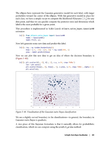
Now we can plot this new data to get an idea of where the decision boundary is
(Figure 5-40):

In[5]: plt.scatter(X[:, 0], X[:, 1], c=y, s=50, cmap='RdBu')
lim = plt.axis()
plt.scatter(Xnew[:, 0], Xnew[:, 1], c=ynew, s=20, cmap='RdBu', alpha=0.1)
plt.axis(lim);

Figure 5-40. Visualization of the Gaussian naive Bayes classification

We see a slightly curved boundary in the classifications—in general, the boundary in
Gaussian naive Bayes is quadratic.
A nice piece of this Bayesian formalism is that it naturally allows for probabilistic
classification, which we can compute using the predict_proba method:

In Depth: Naive Bayes Classification | 385