Page 414 - Python Data Science Handbook

return self._gauss_basis(X[:, :, np.newaxis], self.centers_,
self.width_, axis=1)

gauss_model = make_pipeline(GaussianFeatures(20),
LinearRegression())
gauss_model.fit(x[:, np.newaxis], y)
yfit = gauss_model.predict(xfit[:, np.newaxis])

plt.scatter(x, y)
plt.plot(xfit, yfit)
plt.xlim(0, 10);

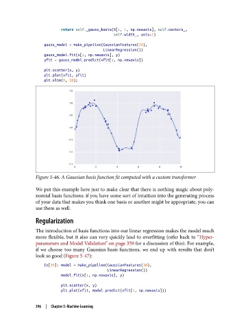
Figure 5-46. A Gaussian basis function fit computed with a custom transformer

We put this example here just to make clear that there is nothing magic about poly‐
nomial basis functions: if you have some sort of intuition into the generating process
of your data that makes you think one basis or another might be appropriate, you can
use them as well.

Regularization

The introduction of basis functions into our linear regression makes the model much
more flexible, but it also can very quickly lead to overfitting (refer back to “Hyper‐
parameters and Model Validation” on page 359 for a discussion of this). For example,
if we choose too many Gaussian basis functions, we end up with results that don’t
look so good (Figure 5-47):

In[10]: model = make_pipeline(GaussianFeatures(30),
LinearRegression())
model.fit(x[:, np.newaxis], y)
plt.scatter(x, y)
plt.plot(xfit, model.predict(xfit[:, np.newaxis]))

396 | Chapter 5: Machine Learning