Page 511 - Python Data Science Handbook

for i, offset in enumerate([0.0, 0.6]):
ax[i].hist(x, bins=bins + offset, normed=True)
ax[i].plot(x, np.full_like(x, -0.01), '|k',
markeredgewidth=1)

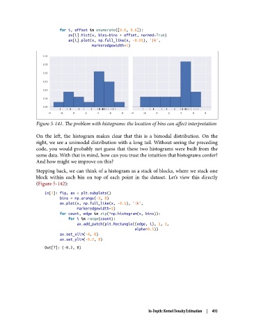
Figure 5-141. The problem with histograms: the location of bins can affect interpretation

On the left, the histogram makes clear that this is a bimodal distribution. On the
right, we see a unimodal distribution with a long tail. Without seeing the preceding
code, you would probably not guess that these two histograms were built from the
same data. With that in mind, how can you trust the intuition that histograms confer?
And how might we improve on this?
Stepping back, we can think of a histogram as a stack of blocks, where we stack one
block within each bin on top of each point in the dataset. Let’s view this directly
(Figure 5-142):
In[7]: fig, ax = plt.subplots()
bins = np.arange(-3, 8)
ax.plot(x, np.full_like(x, -0.1), '|k',
markeredgewidth=1)
for count, edge in zip(*np.histogram(x, bins)):
for i in range(count):
ax.add_patch(plt.Rectangle((edge, i), 1, 1,
alpha=0.5))
ax.set_xlim(-4, 8)
ax.set_ylim(-0.2, 8)
Out[7]: (-0.2, 8)

In-Depth: Kernel Density Estimation | 493