Page 515 - Python Data Science Handbook

kernel bandwidth, which is a free parameter, using Scikit-Learn’s standard cross-
validation tools, as we will soon see.
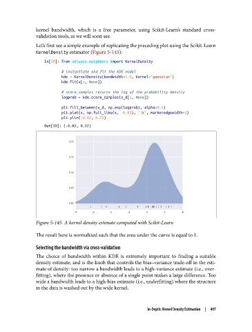
Let’s first see a simple example of replicating the preceding plot using the Scikit-Learn
KernelDensity estimator (Figure 5-145):

In[10]: from sklearn.neighbors import KernelDensity
# instantiate and fit the KDE model
kde = KernelDensity(bandwidth=1.0, kernel='gaussian')
kde.fit(x[:, None])
# score_samples returns the log of the probability density
logprob = kde.score_samples(x_d[:, None])
plt.fill_between(x_d, np.exp(logprob), alpha=0.5)
plt.plot(x, np.full_like(x, -0.01), '|k', markeredgewidth=1)
plt.ylim(-0.02, 0.22)
Out[10]: (-0.02, 0.22)

Figure 5-145. A kernel density estimate computed with Scikit-Learn

The result here is normalized such that the area under the curve is equal to 1.

Selecting the bandwidth via cross-validation
The choice of bandwidth within KDE is extremely important to finding a suitable
density estimate, and is the knob that controls the bias–variance trade-off in the esti‐
mate of density: too narrow a bandwidth leads to a high-variance estimate (i.e., over‐
fitting), where the presence or absence of a single point makes a large difference. Too
wide a bandwidth leads to a high-bias estimate (i.e., underfitting) where the structure
in the data is washed out by the wide kernel.

In-Depth: Kernel Density Estimation | 497