Page 510 - Python Data Science Handbook

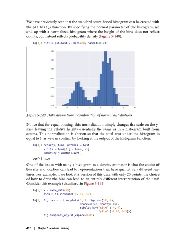
We have previously seen that the standard count-based histogram can be created with
the plt.hist() function. By specifying the normed parameter of the histogram, we
end up with a normalized histogram where the height of the bins does not reflect
counts, but instead reflects probability density (Figure 5-140):

In[3]: hist = plt.hist(x, bins=30, normed=True)

Figure 5-140. Data drawn from a combination of normal distributions

Notice that for equal binning, this normalization simply changes the scale on the y-
axis, leaving the relative heights essentially the same as in a histogram built from
counts. This normalization is chosen so that the total area under the histogram is
equal to 1, as we can confirm by looking at the output of the histogram function:
In[4]: density, bins, patches = hist
widths = bins[1:] - bins[:-1]
(density * widths).sum()
Out[4]: 1.0
One of the issues with using a histogram as a density estimator is that the choice of
bin size and location can lead to representations that have qualitatively different fea‐
tures. For example, if we look at a version of this data with only 20 points, the choice
of how to draw the bins can lead to an entirely different interpretation of the data!
Consider this example (visualized in Figure 5-141):

In[5]: x = make_data(20)
bins = np.linspace(-5, 10, 10)
In[6]: fig, ax = plt.subplots(1, 2, figsize=(12, 4),
sharex=True, sharey=True,
subplot_kw={'xlim':(-4, 9),
'ylim':(-0.02, 0.3)})
fig.subplots_adjust(wspace=0.05)

492 | Chapter 5: Machine Learning