Page 514 - Python Data Science Handbook

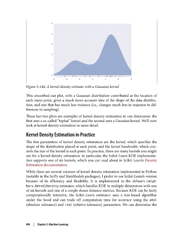
Figure 5-144. A kernel density estimate with a Gaussian kernel

This smoothed-out plot, with a Gaussian distribution contributed at the location of
each input point, gives a much more accurate idea of the shape of the data distribu‐
tion, and one that has much less variance (i.e., changes much less in response to dif‐
ferences in sampling).
These last two plots are examples of kernel density estimation in one dimension: the
first uses a so-called “tophat” kernel and the second uses a Gaussian kernel. We’ll now
look at kernel density estimation in more detail.

Kernel Density Estimation in Practice

The free parameters of kernel density estimation are the kernel, which specifies the
shape of the distribution placed at each point, and the kernel bandwidth, which con‐
trols the size of the kernel at each point. In practice, there are many kernels you might
use for a kernel density estimation: in particular, the Scikit-Learn KDE implementa‐
tion supports one of six kernels, which you can read about in Scikit-Learn’s Density
Estimation documentation.
While there are several versions of kernel density estimation implemented in Python
(notably in the SciPy and StatsModels packages), I prefer to use Scikit-Learn’s version
because of its efficiency and flexibility. It is implemented in the sklearn.neigh
bors.KernelDensity estimator, which handles KDE in multiple dimensions with one
of six kernels and one of a couple dozen distance metrics. Because KDE can be fairly
computationally intensive, the Scikit-Learn estimator uses a tree-based algorithm
under the hood and can trade off computation time for accuracy using the atol
(absolute tolerance) and rtol (relative tolerance) parameters. We can determine the

496 | Chapter 5: Machine Learning