Page 98 - Python Data Science Handbook

for example, if we combine a column vector and a row vector within the indices, we
get a two-dimensional result:

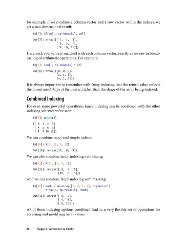
In[7]: X[row[:, np.newaxis], col]
Out[7]: array([[ 2, 1, 3],
[ 6, 5, 7],
[10, 9, 11]])
Here, each row value is matched with each column vector, exactly as we saw in broad‐
casting of arithmetic operations. For example:
In[8]: row[:, np.newaxis] * col
Out[8]: array([[0, 0, 0],
[2, 1, 3],
[4, 2, 6]])
It is always important to remember with fancy indexing that the return value reflects
the broadcasted shape of the indices, rather than the shape of the array being indexed.

Combined Indexing

For even more powerful operations, fancy indexing can be combined with the other
indexing schemes we’ve seen:

In[9]: print(X)
[[ 0 1 2 3]
[ 4 5 6 7]
[ 8 9 10 11]]
We can combine fancy and simple indices:

In[10]: X[2, [2, 0, 1]]
Out[10]: array([10, 8, 9])
We can also combine fancy indexing with slicing:
In[11]: X[1:, [2, 0, 1]]
Out[11]: array([[ 6, 4, 5],
[10, 8, 9]])
And we can combine fancy indexing with masking:

In[12]: mask = np.array([1, 0, 1, 0], dtype=bool)
X[row[:, np.newaxis], mask]
Out[12]: array([[ 0, 2],
[ 4, 6],
[ 8, 10]])
All of these indexing options combined lead to a very flexible set of operations for
accessing and modifying array values.

80 | Chapter 2: Introduction to NumPy