Page 896 - Elementary_Linear_Algebra_with_Applications_Anton__9_edition

EXAMPLE 4 Example 1 Revisited
The transition matrix in Example 1 was

If a car is rented initially from location 2, then the initial state vector is

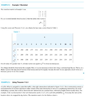
Using this vector and Theorem 11.6.1, one obtains the later state vectors listed in Table 1.

Table 1

n

0 1 2 3 4 5 6 7 8 9 10 11

0 .300 .400 .477 .511 .533 .544 .550 .553 .555 .556 .557
1 .200 .370 .252 .261 .240 .238 .233 .232 .231 .230 .230
0 .500 .230 .271 .228 .227 .219 .217 .215 .214 .214 .213
For all values of n greater than 11, all state vectors are equal to to three decimal places.
Two things should be observed in this example. First, it was not necessary to know how long a customer kept the car. That is, in a
Markov process the time period between observations need not be regular. Second, the state vectors approach a fixed vector as n
increases, just as in the first example.

EXAMPLE 5 Using Theorem 11.6.1
A traffic officer is assigned to control the traffic at the eight intersections indicated in Figure 11.6.1. She is instructed to remain at
each intersection for an hour and then to either remain at the same intersection or move to a neighboring intersection. To avoid
establishing a pattern, she is told to choose her new intersection on a random basis, with each possible choice equally likely. For
example, if she is at intersection 5, her next intersection can be 2, 4, 5, or 8, each with probability . Every day she starts at the
location where she stopped the day before. The transition matrix for this Markov chain is