Page 58 - Class-11-Physics-Part-1_Neat

44 PHYSICS

calculation. Let us take ∆t = 2 s centred at instant for motion of the car shown in Fig. 3.3.
t = 4 s. Then, by the definition of the average For this case, the variation of velocity with time
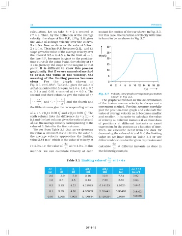
velocity, the slope of line P P ( Fig. 3.6) gives is found to be as shown in Fig. 3.7.
1 2
the value of average velocity over the interval
3 s to 5 s. Now, we decrease the value of ∆t from
2 s to 1 s. Then line P P becomes Q Q and its
1 2 1 2
slope gives the value of the average velocity over
the interval 3.5 s to 4.5 s. In the limit ∆t → 0,
the line P P becomes tangent to the position-
1 2
time curve at the point P and the velocity at t =
4 s is given by the slope of the tangent at that
point. It is difficult to show this process
graphically. But if we use numerical method
to obtain the value of the velocity, the
meaning of the limiting process becomes
clear. For the graph shown in
3
Fig. 3.6, x = 0.08 t . Table 3.1 gives the value of
∆x/∆t calculated for ∆t equal to 2.0 s, 1.0 s, 0.5
s, 0.1 s and 0.01 s centred at t = 4.0 s. The
Fig. 3.7 Velocity–time graph corresponding to motion
second and third columns give the value of t =
1 shown in Fig. 3.3.
 ∆ t   ∆ t  The graphical method for the determination
 t −  and t 2 =  t +  and the fourth and
 2   2  of the instantaneous velocity is always not a
the fifth columns give the corresponding values convenient method. For this, we must carefully
plot the position–time graph and calculate the
3 3
of x, i.e. x (t ) = 0.08 t and x (t ) = 0.08 t . The value of average velocity as ∆t becomes smaller
1 1 2 2
sixth column lists the difference ∆x = x (t ) – x and smaller. It is easier to calculate the value
2
(t ) and the last column gives the ratio of ∆x and of velocity at different instants if we have data
1
∆t, i.e. the average velocity corresponding to the of positions at different instants or exact
value of ∆t listed in the first column. expression for the position as a function of time.
We see from Table 3.1 that as we decrease Then, we calculate ∆x/∆t from the data for
the value of ∆t from 2.0 s to 0.010 s, the value of decreasing the value of ∆t and find the limiting
the average velocity approaches the limiting value as we have done in Table 3.1 or use
–1
value 3.84 m s which is the value of velocity at differential calculus for the given expression and
dx dx
t = 4.0 s, i.e. the value of at t = 4.0 s. In this calculate at different instants as done in
dt dt
manner, we can calculate velocity at each the following example.

∆x
Table 3.1 Limiting value of at t = 4 s
∆t

2018-19