Page 166 - Applied Statistics with R

166 CHAPTER 9. MULTIPLE LINEAR REGRESSION

⊤ ̂
̂ ( ) =
0
0
̂
̂
̂
̂

= + + + ⋯ + −1 0( −1) .
0
2 02
1 01
As with SLR, this is an unbiased estimate.
⊤

E[ ̂( )] =
0
0

= + + + ⋯ + −1 0( −1)
0
1 01
2 02
To make an interval estimate, we will also need its standard error.
SE[ ̂( )] = √ ⊤ ⊤ −1 0
( )

0
0
Putting it all together, we obtain a confidence interval for the mean response.
̂ ( ) ± /2, − ⋅ √ ⊤ ⊤ −1 0
( )
0
0
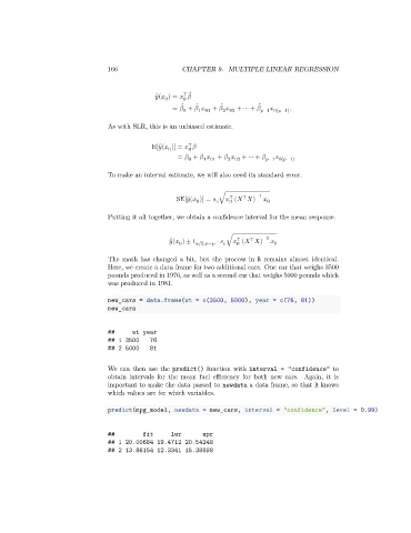
The math has changed a bit, but the process in R remains almost identical.
Here, we create a data frame for two additional cars. One car that weighs 3500
pounds produced in 1976, as well as a second car that weighs 5000 pounds which
was produced in 1981.
new_cars = data.frame(wt = c(3500, 5000), year = c(76, 81))
new_cars

## wt year
## 1 3500 76
## 2 5000 81

We can then use the predict() function with interval = "confidence" to
obtain intervals for the mean fuel efficiency for both new cars. Again, it is
important to make the data passed to newdata a data frame, so that R knows
which values are for which variables.

predict(mpg_model, newdata = new_cars, interval = "confidence", level = 0.99)

## fit lwr upr
## 1 20.00684 19.4712 20.54248
## 2 13.86154 12.3341 15.38898