Page 220 - Applied Statistics with R

220 CHAPTER 11. CATEGORICAL PREDICTORS AND INTERACTIONS

This looks much better! We can see that for medium displacement cars, 6
cylinder cars now perform better than 8 cylinder cars, which seems much more
reasonable than before.
To completely justify the interaction model (i.e., a unique slope for each cyl
level) compared to the additive model (single slope), we can perform an -test.
Notice first, that there is no -test that will be able to do this since the difference
between the two models is not a single parameter.
We will test,

∶ = = 0
3
2
0
which represents the parallel regression lines we saw before,

= + + + + .
1
3 3
2 2
0
Again, this is a difference of two parameters, thus no -test will be useful.
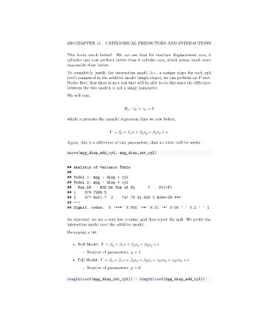
anova(mpg_disp_add_cyl, mpg_disp_int_cyl)

## Analysis of Variance Table
##
## Model 1: mpg ~ disp + cyl
## Model 2: mpg ~ disp * cyl
## Res.Df RSS Df Sum of Sq F Pr(>F)
## 1 379 7299.5
## 2 377 6551.7 2 747.79 21.515 1.419e-09 ***
## ---
## Signif. codes: 0 '***' 0.001 '**' 0.01 '*' 0.05 '.' 0.1 ' ' 1

As expected, we see a very low p-value, and thus reject the null. We prefer the
interaction model over the additive model.
Recapping a bit:

• Null Model: = + + + +
3 3
2 2
0
1
– Number of parameters: = 4
• Full Model: = + + + + + +
2
3
2
3 3
0
3
2 2
1
– Number of parameters: = 6
length(coef(mpg_disp_int_cyl)) - length(coef(mpg_disp_add_cyl))