Page 219 - Applied Statistics with R

11.3. FACTOR VARIABLES 219

̂
• ( + ̂ ) = −0.1306935+0.1081714 = −0.0225221 is the estimated change

3
1
in average mpg for an increase of one disp, for an 8 cylinder car.
So, as we have seen before and change the intercepts for 6 and 8 cylinder
3
2
cars relative to the reference level of for 4 cylinder cars.
0
Now, similarly and change the slopes for 6 and 8 cylinder cars relative to
3
2
the reference level of for 4 cylinder cars.
1
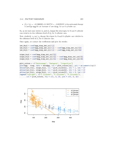
Once again, we extract the coefficients and plot the results.
int_4cyl = coef(mpg_disp_int_cyl)[1]
int_6cyl = coef(mpg_disp_int_cyl)[1] + coef(mpg_disp_int_cyl)[3]
int_8cyl = coef(mpg_disp_int_cyl)[1] + coef(mpg_disp_int_cyl)[4]
slope_4cyl = coef(mpg_disp_int_cyl)[2]
slope_6cyl = coef(mpg_disp_int_cyl)[2] + coef(mpg_disp_int_cyl)[5]
slope_8cyl = coef(mpg_disp_int_cyl)[2] + coef(mpg_disp_int_cyl)[6]

plot_colors = c("Darkorange", "Darkgrey", "Dodgerblue")
plot(mpg ~ disp, data = autompg, col = plot_colors[cyl], pch = as.numeric(cyl))
abline(int_4cyl, slope_4cyl, col = plot_colors[1], lty = 1, lwd = 2)
abline(int_6cyl, slope_6cyl, col = plot_colors[2], lty = 2, lwd = 2)
abline(int_8cyl, slope_8cyl, col = plot_colors[3], lty = 3, lwd = 2)
legend("topright", c("4 Cylinder", "6 Cylinder", "8 Cylinder"),
col = plot_colors, lty = c(1, 2, 3), pch = c(1, 2, 3))

4 Cylinder
6 Cylinder
40 8 Cylinder

mpg 30

20

10

100 200 300 400
disp