Page 327 - Applied Statistics with R

14.2. PREDICTOR TRANSFORMATION 327

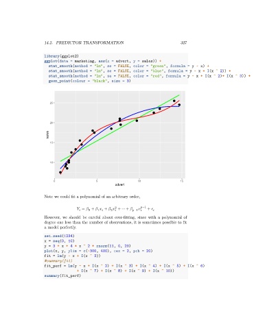
library(ggplot2)
ggplot(data = marketing, aes(x = advert, y = sales)) +
stat_smooth(method = "lm", se = FALSE, color = "green", formula = y ~ x) +
stat_smooth(method = "lm", se = FALSE, color = "blue", formula = y ~ x + I(x ^ 2)) +
stat_smooth(method = "lm", se = FALSE, color = "red", formula = y ~ x + I(x ^ 2)+ I(x ^ 3)) +
geom_point(colour = "black", size = 3)

25

20
sales

15

10

0 5 10 15
advert

Note we could fit a polynomial of an arbitrary order,

2
= + + + ⋯ + −1 −1 +

2
1
0

However, we should be careful about over-fitting, since with a polynomial of
degree one less than the number of observations, it is sometimes possible to fit
a model perfectly.
set.seed(1234)
x = seq(0, 10)
y = 3 + x + 4 * x ^ 2 + rnorm(11, 0, 20)
plot(x, y, ylim = c(-300, 400), cex = 2, pch = 20)
fit = lm(y ~ x + I(x ^ 2))
#summary(fit)
fit_perf = lm(y ~ x + I(x ^ 2) + I(x ^ 3) + I(x ^ 4) + I(x ^ 5) + I(x ^ 6)
+ I(x ^ 7) + I(x ^ 8) + I(x ^ 9) + I(x ^ 10))
summary(fit_perf)