Page 369 - Applied Statistics with R

15.2. COLLINEARITY 369

100 200 300 150 180 26 32 38 30 36 42
60
Age
40
20
300
200 Weight
100
190
HtShoes
160

180 Ht
150
100
Seated 90
80
38
32 Arm
26
45
Thigh
35
42
36 Leg
30
-100
hipcenter
-250
20 40 60 160 190 80 90 100 35 45 -250 -100

round(cor(seatpos), 2)

## Age Weight HtShoes Ht Seated Arm Thigh Leg hipcenter
## Age 1.00 0.08 -0.08 -0.09 -0.17 0.36 0.09 -0.04 0.21
## Weight 0.08 1.00 0.83 0.83 0.78 0.70 0.57 0.78 -0.64
## HtShoes -0.08 0.83 1.00 1.00 0.93 0.75 0.72 0.91 -0.80
## Ht -0.09 0.83 1.00 1.00 0.93 0.75 0.73 0.91 -0.80
## Seated -0.17 0.78 0.93 0.93 1.00 0.63 0.61 0.81 -0.73
## Arm 0.36 0.70 0.75 0.75 0.63 1.00 0.67 0.75 -0.59
## Thigh 0.09 0.57 0.72 0.73 0.61 0.67 1.00 0.65 -0.59
## Leg -0.04 0.78 0.91 0.91 0.81 0.75 0.65 1.00 -0.79
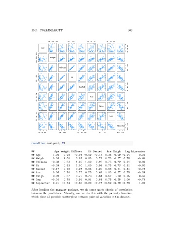
## hipcenter 0.21 -0.64 -0.80 -0.80 -0.73 -0.59 -0.59 -0.79 1.00

After loading the faraway package, we do some quick checks of correlation
between the predictors. Visually, we can do this with the pairs() function,
which plots all possible scatterplots between pairs of variables in the dataset.