Page 373 - Applied Statistics with R

15.2. COLLINEARITY 373

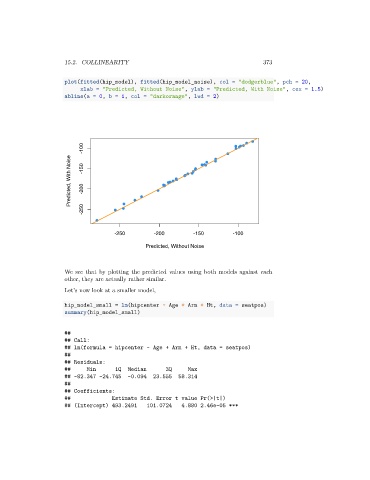
plot(fitted(hip_model), fitted(hip_model_noise), col = "dodgerblue", pch = 20,
xlab = "Predicted, Without Noise", ylab = "Predicted, With Noise", cex = 1.5)
abline(a = 0, b = 1, col = "darkorange", lwd = 2)

-100
Predicted, With Noise -150 -200

-250

-250 -200 -150 -100
Predicted, Without Noise

We see that by plotting the predicted values using both models against each
other, they are actually rather similar.
Let’s now look at a smaller model,

hip_model_small = lm(hipcenter ~ Age + Arm + Ht, data = seatpos)
summary(hip_model_small)

##
## Call:
## lm(formula = hipcenter ~ Age + Arm + Ht, data = seatpos)
##
## Residuals:
## Min 1Q Median 3Q Max
## -82.347 -24.745 -0.094 23.555 58.314
##
## Coefficients:
## Estimate Std. Error t value Pr(>|t|)
## (Intercept) 493.2491 101.0724 4.880 2.46e-05 ***