Page 370 - Applied Statistics with R

370 CHAPTER 15. COLLINEARITY

We can also do this numerically with the cor() function, which when applied to
a dataset, returns all pairwise correlations. Notice this is a symmetric matrix.
Recall that correlation measures strength and direction of the linear relationship
between to variables. The correlation between Ht and HtShoes is extremely
high. So high, that rounded to two decimal places, it appears to be 1!
Unlike exact collinearity, here we can still fit a model with all of the predictors,
but what effect does this have?

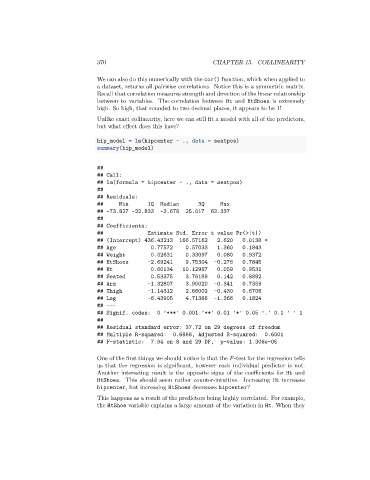
hip_model = lm(hipcenter ~ ., data = seatpos)
summary(hip_model)

##
## Call:
## lm(formula = hipcenter ~ ., data = seatpos)
##
## Residuals:
## Min 1Q Median 3Q Max
## -73.827 -22.833 -3.678 25.017 62.337
##
## Coefficients:
## Estimate Std. Error t value Pr(>|t|)
## (Intercept) 436.43213 166.57162 2.620 0.0138 *
## Age 0.77572 0.57033 1.360 0.1843
## Weight 0.02631 0.33097 0.080 0.9372
## HtShoes -2.69241 9.75304 -0.276 0.7845
## Ht 0.60134 10.12987 0.059 0.9531
## Seated 0.53375 3.76189 0.142 0.8882
## Arm -1.32807 3.90020 -0.341 0.7359
## Thigh -1.14312 2.66002 -0.430 0.6706
## Leg -6.43905 4.71386 -1.366 0.1824
## ---
## Signif. codes: 0 '***' 0.001 '**' 0.01 '*' 0.05 '.' 0.1 ' ' 1
##
## Residual standard error: 37.72 on 29 degrees of freedom
## Multiple R-squared: 0.6866, Adjusted R-squared: 0.6001
## F-statistic: 7.94 on 8 and 29 DF, p-value: 1.306e-05

One of the first things we should notice is that the -test for the regression tells
us that the regression is significant, however each individual predictor is not.
Another interesting result is the opposite signs of the coefficients for Ht and
HtShoes. This should seem rather counter-intuitive. Increasing Ht increases
hipcenter, but increasing HtShoes decreases hipcenter?

This happens as a result of the predictors being highly correlated. For example,
the HtShoe variable explains a large amount of the variation in Ht. When they