Page 371 - Applied Statistics with R

15.2. COLLINEARITY 371

are both in the model, their effects on the response are lessened individually,
but together they still explain a large portion of the variation of hipcenter.
2
We define to be the proportion of observed variation in the -th predictor

2
explained by the other predictors. In other words is the multiple R-Squared

for the regression of on each of the other predictors.

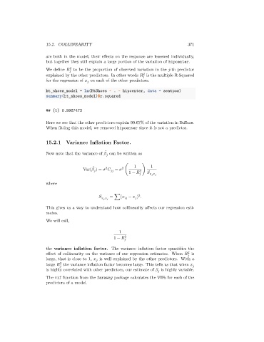
ht_shoes_model = lm(HtShoes ~ . - hipcenter, data = seatpos)
summary(ht_shoes_model)$r.squared

## [1] 0.9967472

Here we see that the other predictors explain 99.67% of the variation in HtShoe.
When fitting this model, we removed hipcenter since it is not a predictor.

15.2.1 Variance Inflation Factor.

̂
Now note that the variance of can be written as

1 1
̂
2
2
Var( ) = = ( 1 − 2 )

where
2
= ∑( − ̄ ) .

This gives us a way to understand how collinearity affects our regression esti-
mates.
We will call,

1
1 − 2

the variance inflation factor. The variance inflation factor quantifies the
2
effect of collinearity on the variance of our regression estimates. When is

large, that is close to 1, is well explained by the other predictors. With a

2
large the variance inflation factor becomes large. This tells us that when

is highly correlated with other predictors, our estimate of is highly variable.

The vif function from the faraway package calculates the VIFs for each of the
predictors of a model.